Loss and Gradient

A model is a function $f_w : \mathbb R^d \to \mathbb R$ or $f_w : \mathbb R^d \to \mathbb R^K$ with adjustable params $w$.

Now when we say a model "learns". Learning refers to choosing good values of $w$. But "good" needs to be a number before anything can be optimised.

Loss is exactly this number which takes the prediction and the true answer and returns a non-negative score of how wrong the predicted value is ($0$ = minimum, which means the prediction is perfect).

Learning becomes :

Everything in machine learning for example, Gradient descent, backprop, training loop is for minimizing the loss.

To describe the loss let's take the example of loss for a single entry from our dataset. Formally, a loss function is a map :

Or we can say that for a set of prediction and actual value $(\hat{y}, y)$ our map becomes :

Also to represent the loss for the whole dataset we will use (this is known as Empirical Risk)

Loss Types

Now there are several ways to represent loss and every type has it's own pros and cons.

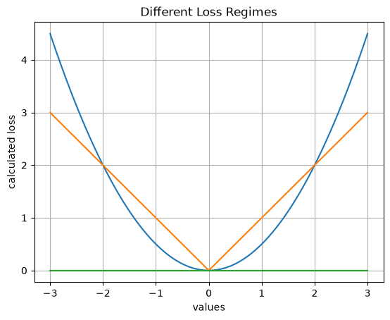
Squared Loss

In this type the penalty grows quadratically with miss distance.

Absolute loss

In this type the penalty grows linearly not quadratically. One of the pros of using this loss is that the outliers in the data pull less hardly when penalty is applied.

0-1 loss

In this type it returns 1 when wrong, 0 when correct (it counts errors).

We can clearly see the problem: This loss is piecewise constant so its gradient is zero wherever it's defined and undefined at the jumps. Gradient descent gets no signal from it because there's no slope pointing toward "less wrong." This is exactly why we need smooth surrogate losses like cross-entropy which is what the next section introduces.

Cross Entropy / Negative Log Likelihood

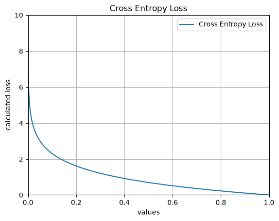
The model outputs a probability distribution $\hat{p} \in \Delta^{K - 1}$ (via softmax) :

Here as $\hat{p}_y$ approaches 0, our loss $\ell$ approaches $\infty$.

Where Do These Losses Come From?

Almost every standard loss is the same object in disguise: the negative log-likelihood of the data under an assumed noise model.

The recipe has three steps:

1. Assume a probability model for the label given the input: $p(y \mid x; w)$.
2. Maximize likelihood pick $w$ making the observed data most probable: $\max_{w}\; \prod_{i=1}^{n} p(y_i \mid x_i; w)$
3. Take $-\log$, the logarithm is monotonic (so it doesn't move the maximizer) and it turns the product into a sum and the max into a min: $w_{\text{MLE}} = \underset{w}{\arg\min}\; \sum_{i=1}^{n} -\log p(y_i \mid x_i; w)$

Compare this to $\mathcal{L}(w) = \frac{1}{n}\sum_{i} \ell(\hat{y}_i, y_i)$: the per example loss is the negative log likelihood, $\ell = -\log p(y_i \mid x_i; w)$.

Gaussian noise gives squared loss. If you assume the label is the model's prediction plus bell-curve noise, minimizing squared error is exactly maximum likelihood. This is why least-squares is everywhere and that's why it's outlier-sensitive. The Gaussian assigns tiny probability to large deviations so the fit distorts to avoid them.

Categorical labels give cross-entropy. If you assume the label is drawn from a categorical distribution whose probabilities are the model's softmax outputs, the negative log-likelihood is precisely $-\log \hat{p}_y$ which is the cross-entropy from the previous section.

Gradients

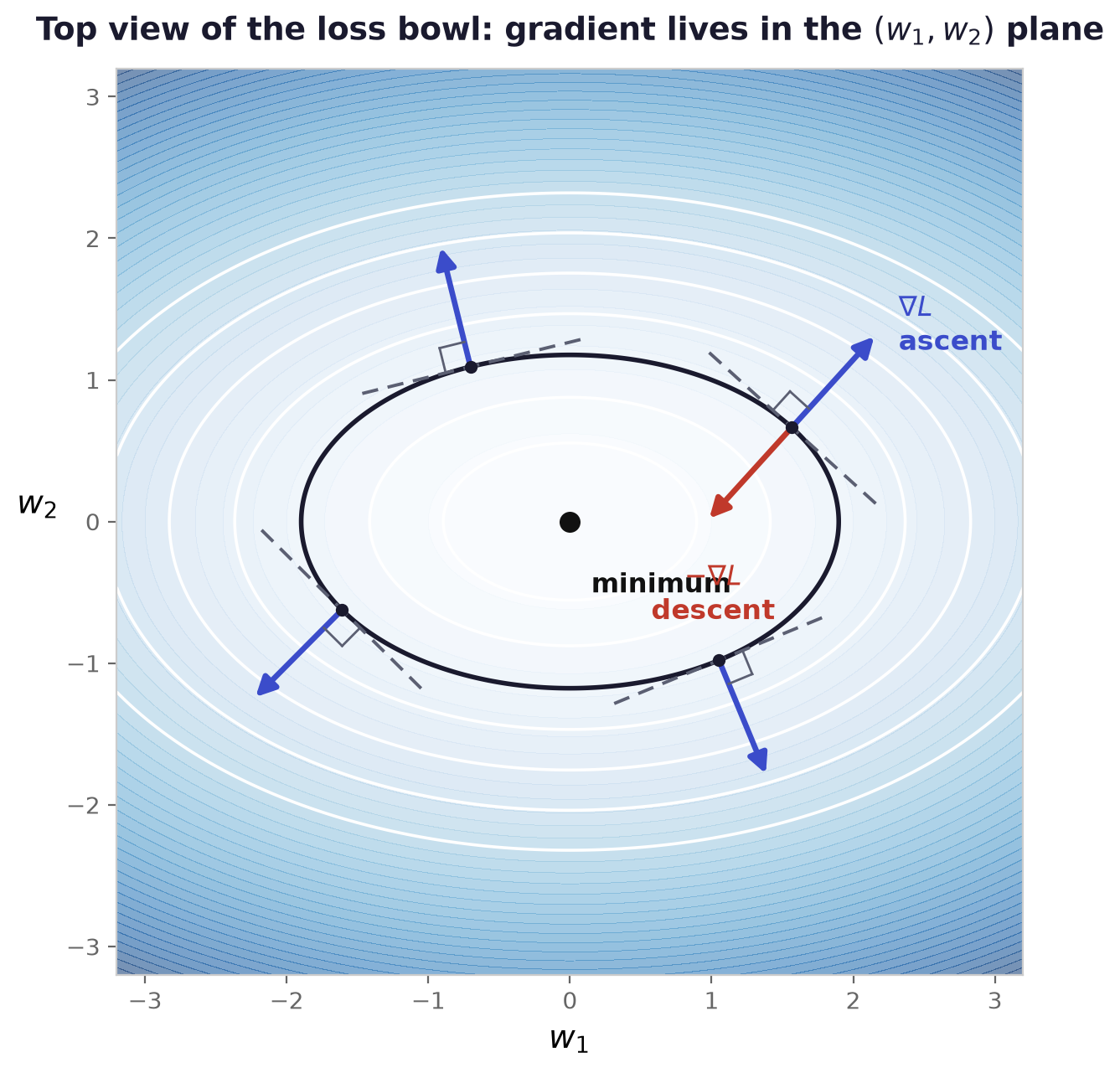
We now have a loss $\mathcal{L}(w)$ and a goal which is to minimize it. To "minimize" is kind of unclear. To actually move the weights toward a smaller loss, we need to know, at our current $w$, which way is downhill. That direction is what the gradient gives us.

Notation from here on. We are moving into vectors and matrices. Bold lowercase letters ($\mathbf{w}, \mathbf{x}, \mathbf{h}$) are vectors; capitals ($X, H, Q$) are matrices; plain lowercase ($\eta, \lambda, \kappa$) are scalars. A subscript picks out an entry: $w_j$ is the $j$-th component of $\mathbf{w}$.

One dimension: the derivative

For a function of a single variable $L(w)$, the derivative is the local slope:

It answers: if I nudge $w$ a little, how fast does $L$ change? It carries two pieces of info :

• its sign tells you the direction of increase (positive slope means increasing $w$ increases $L$)
• its magnitude tells you how sensitive $L$ is to that nudge.

Many dimensions: partial derivatives

Now let $L : \mathbb{R}^d \to \mathbb{R}$ be the loss as a function of all $d$ weights $\mathbf{w} = (w_1, \dots, w_d)^\top$. There is no single "slope" anymore, because from any point you can move in infinitely many directions. But you can still ask the one-dimensional question one coordinate at a time:

In words: hold every weight fixed except $w_j$, nudge only $w_j$, measure the response. That is a partial derivative which one number per coordinate.

The mechanic in practice is to treat every other variable as a constant. For example, with $L(w_1, w_2) = w_1^2 + 3 w_1 w_2$:

Stacking them: the gradient

The gradient collects all $d$ partial derivatives into a single vector:

Why this particular vector matters

The gradient compresses all directional information into one object. Take a small step $\mathbf{h}$ from $\mathbf{w}$ and ask how $L$ changes. The first-order Taylor expansion says:

So the change in $L$ under any direction of movement is just an inner product with the gradient. Now use the geometric form of the inner product, $\nabla L^\top \mathbf{h} = \|\nabla L\|\,\|\mathbf{h}\|\cos\theta$, and sweep over all unit directions $\mathbf{h}$:

• $L$ increases fastest when $\theta = 0$ that is, in the direction of $\nabla L$ itself. So the gradient points in the direction of steepest ascent, and $\|\nabla L\|$ is that maximal rate of increase.
• $L$ decreases fastest when $\theta = \pi$ the direction $-\nabla L$. This is steepest descent, and it is exactly the direction we will step in next.
• Directions with $\theta = \pi/2$ (perpendicular to the gradient) leave $L$ unchanged to first order. In other words, the gradient is orthogonal to the level sets (the contour lines of constant loss). That last fact is worth holding onto — every contour picture for the rest of this post is readable because the gradient always crosses the contours at right angles.

One consequence: at a minimum, no direction decreases $L$, which forces

"Minimizing the loss" concretely means "finding where the gradient is zero."

Gradient Descent

The gradient hands us a downhill direction at every point. Gradient descent is nothing more than: stand where you are, look at $-\nabla L$, take a step that way, repeat.

$\nabla L(\mathbf{w}_t)$ is the locally steepest uphill direction; the minus sign flips it downhill; $\eta$ (the learning rate) scales how far we move; and we repeat until $\nabla L \approx \mathbf{0}$, i.e. until no direction goes downhill anymore.

The learning rate is delicate

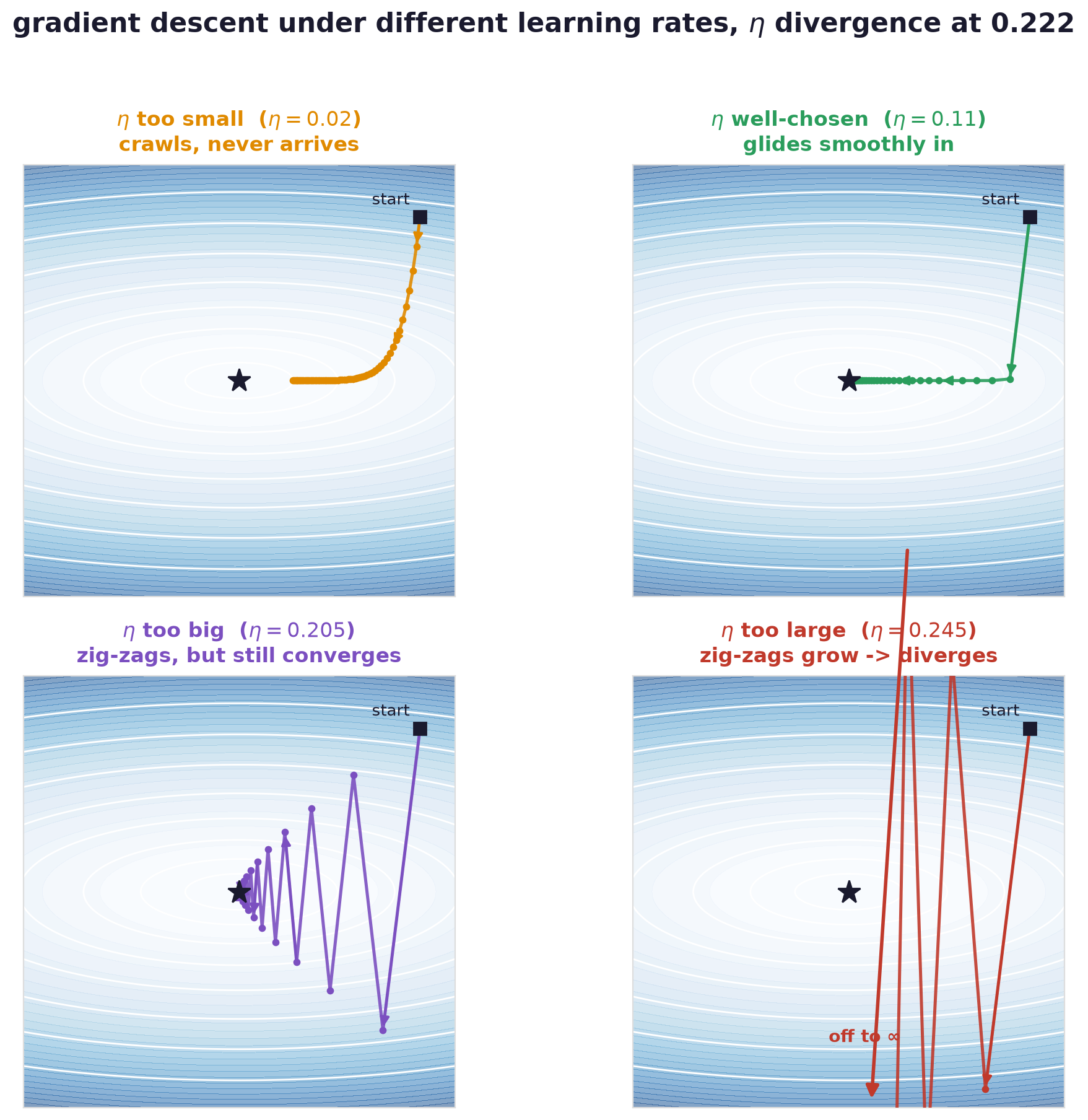
That single number $\eta$ controls everything, and picking it badly breaks training. On the same loss surface, four regimes:

• Too small. The steps are tiny; the iterates crawl toward the minimum and waste thousands of steps getting there.
• Well-chosen. The iterates glide smoothly down into the minimum in a handful of steps.
• Too big. Each step overshoots the bottom and lands on the far wall; the path zig-zags across the valley, making slow progress at best.
• Way too big. The overshoot grows every step. The iterates spiral outward and the loss diverges to infinity.

Personal To Study Note (Not part of the main article) :warning: 🚨 AI GENERATED CONTENT (NOT VERIFIED) 🚨 :warning:

Why Speed Varies: Conditioning

Here is the question from the last section, sharpened: why does the same algorithm need ten steps on one problem and ten thousand on another? The answer is the shape of the loss surface, and for least-squares we can work it out exactly.

Least-squares is an exact quadratic bowl

Take linear regression with squared loss. Writing the predictions as $X\mathbf{w}$ (the design matrix $X$ times the weights):

Expand and differentiate using the two identities from earlier (this is where the $\frac{1}{2}$ we carried since the squared-loss definition it cancels the 2 from the derivative):

Differentiate once more to get the Hessian which is the matrix of second partial derivatives, i.e. the derivative of the gradient:

Notice what did not happen: $H$ has no $\mathbf{w}$ in it. The Hessian is constant. That means $\mathcal{L}$ is exactly a quadratic function — a $d$-dimensional paraboloid, a bowl — with no approximation anywhere. (For a neural network the loss isn't globally quadratic, but near a minimum this same analysis applies via a second-order Taylor expansion. Mastering the linear case is how you understand the general one.)

The minimizer, and the gradient rewritten around it

Setting $\nabla \mathcal{L} = \mathbf{0}$ gives the Normal Equation:

Now a small trick that makes everything downstream trivial. Since $X^\top \mathbf{y} = X^\top X \mathbf{w}^*$, substitute it back into the gradient:

The gradient is a linear function of the error $\mathbf{w} - \mathbf{w}^*$. Hold onto this line — it's the engine of the whole argument.

Eigenvalues are the curvatures of the bowl

$H = \frac{1}{n}X^\top X$ is symmetric and positive (semi-)definite, so by the spectral theorem it has an orthonormal eigendecomposition:

where the columns $\mathbf{q}_1, \dots, \mathbf{q}_d$ of $Q$ are orthonormal eigenvectors. What does an eigenvalue mean here? Step a distance $t$ away from the minimum along eigendirection $\mathbf{q}_i$ and measure the loss (exact, since $\mathcal{L}$ is quadratic):

So along $\mathbf{q}_i$ the loss is a 1-D parabola with curvature $\lambda_i$. Large $\lambda_i$ = steep, tight valley wall; small $\lambda_i$ = nearly flat floor. The level sets $\{\mathbf{w} : \mathcal{L}(\mathbf{w}) = c\}$ are ellipsoids whose axis along $\mathbf{q}_i$ has length proportional to $1/\sqrt{\lambda_i}$. If $\lambda_1 = 10^6$ and $\lambda_2 = 1$, the ellipse is $1000\times$ longer in one direction than the other — a long, narrow ravine.

The condition number measures exactly this lopsidedness — the ratio of steepest to shallowest curvature:

$\kappa = 1$ is a perfectly round bowl; $\kappa = 10^6$ is a pathological ravine.

Gradient descent decouples, one eigendirection at a time

Now run gradient descent on this bowl and watch the error evolve. Start from the update rule, substitute the error-form of the gradient, and define the error $\mathbf{e}_t := \mathbf{w}_t - \mathbf{w}^*$:

The error just gets multiplied by the fixed matrix $I - \eta H$ every step. Change basis to the eigenvectors — let $\tilde{e}_t^{(i)} = \mathbf{q}_i^\top \mathbf{e}_t$ be the component of the error along eigendirection $i$. Because $Q^\top (I - \eta H) Q = I - \eta \Lambda$ is diagonal, the directions stop interacting:

This is the whole story in one line. Gradient descent on a quadratic decouples into $d$ independent 1-D problems, one per eigendirection, each shrinking geometrically at its own rate $|1 - \eta \lambda_i|$. There is no cross-talk between directions.

The divergence cliff, explained

Direction $i$ converges if and only if $|1 - \eta \lambda_i| < 1$, which rearranges to $0 < \eta < 2/\lambda_i$. This must hold for every direction at once, and the binding constraint is the largest eigenvalue:

There is the cliff from the previous section. If $\eta \ge 2/\lambda_{\max}$, the component along the steepest direction $\mathbf{q}_1$ has $|1 - \eta \lambda_{\max}| \ge 1$, so it fails to shrink — it oscillates with non-decreasing amplitude and the iterates bounce up the ravine walls, higher each time. Divergence is caused entirely by the steepest direction. The "way too big" regime wasn't mysterious; it was $\eta$ crossing $2/\lambda_{\max}$.

The speed limit

Here's the tension. You'd love to crank $\eta$ up to make the slowest direction (rate $|1 - \eta\lambda_{\min}|$) converge faster — but the steep direction caps you at $\eta < 2/\lambda_{\max}$. The best you can do is balance them. Minimizing the worst-case contraction rate over all directions gives the optimal step size and rate:

iterations. The number of steps scales linearly with the condition number. $\kappa = 10^6$ means on the order of a million iterations where a round bowl ($\kappa \approx 1$) would take a handful. That is the precise, quantitative reason "some problems train in ten steps and others in ten thousand."

Now the payoff. Where does a large $\kappa$ actually come from? Look at the entries of $H = \frac{1}{n}X^\top X$:

The diagonal entry $H_{jj}$ is the mean squared magnitude of feature $j$. Feature scales sit directly on the Hessian's diagonal. Take two uncorrelated features — house size ($\sim 10^3$, so $H_{11} \approx 10^6$) and bedroom count ($\sim 3$, so $H_{22} \approx 10$). With no correlation, $H$ is diagonal, its eigenvalues are those diagonal entries, and

The ravine — and the resulting ten-thousand-step slog — comes entirely from the two features being measured in different units.

Standardization fixes exactly this. After rescaling every feature to mean 0 and variance 1, each diagonal entry becomes $H_{jj} = 1$, and $\frac{1}{n}X^\top X$ becomes the feature correlation matrix. If the features are roughly uncorrelated that's approximately the identity, whose eigenvalues are all 1 — so $\kappa \approx 1$, a round bowl, and gradient descent converges almost immediately. This is the whole reason normalization speeds up training: it collapses the condition number. Not folklore — a theorem about the Hessian's eigenvalues.

Honest caveat. Standardization equalizes the diagonal but does not remove correlations (the off-diagonal terms). Two highly correlated features still produce a large $\kappa$: for correlation $r$, the $2\times 2$ correlation matrix has eigenvalues $1 + r$ and $1 - r$, so $\kappa = \frac{1+r}{1-r} \to \infty$ as $r \to 1$. Fully fixing that needs whitening (rotate into the eigenbasis and rescale), which is usually too expensive to bother with. Standardization is the cheap fix that kills the scale-induced part of the ill-conditioning — in practice, usually the dominant part.